The Wave Equation

d’Alembert’s equation

d’Alembert’s equation gives the solution of the homogeneous wave equation \(u_{xx}-c^2u_{tt}=0\) subject to initial conditions that define the original displacement profile (that is \(u(x,0)=f(x)\)) and an initial velocity profile \(\text{(i.e. }u_t(x,0)=g(x)\text{).}\) The solution is then given by

\[\begin{split} \begin{aligned} u(x,t) &= \frac{1}{2}\!\left(f(x+ct)+f(x-ct)\right) \\ &\qquad + \frac{1}{2c}\int_{x-ct}^{x+ct} g(\lambda)\,d\lambda. \end{aligned} \end{split}\]

Such a problem with initial conditions is known as a Cauchy problem.

Derivation of d’Alembert’s equation

Derivation of d’Alembert’s equation

Solution on a finite-length string

The wave equation on a finite-length string with suitable initial and boundary conditions (e.g. fixed endpoints) is an example of a Sturm-Liouville problem. It can be solved by seeking a separable solution in the form

\[ u(x,t)=X(x)T(t). \]

Substituting this assumed form into the PDE and rearranging, one can reduce the problem to two second order ODEs, one for \(X(x)\) and another for \(T(t)\). This arises since one side of the resulting ODE is a function of \(t\) only, while the other is a function only of \(x\); since these are independent variables it must be true that both sides are equal to a constant. Upon solving the problem for \(X(x)\) we’ll usually discover that non-trivial solutions only exist for certain values of the aforementioned constant. We call such values eigenvalues.

The superposition principle allows us to write the solution in the form of an infinite series. We then use Fourier series in order to determine coefficients in the general solution that enable initial conditions to be satisfied.

See your notes from the lectures for the detail.

Duhamel’s equation - inhomogeneous wave equation

The inhomogeneous one-dimensional wave equation is given by

\[ u_{tt}-c^2u_{xx}=h(x,t). \]

The presence of the function \(h(x,t)\) models a source of waves.

In the lectures we’ve seen that the solution to the inhomogeneous wave equations with homogeneous initial conditions

\[ u(x,0)=0, \]

\[ u_t(x,0)=0, \]

is given by

\[ u(x,t)=\frac{1}{2c}\int\limits_{0}^t\int\limits_{x-c(t-\tau)}^{x+c(t-\tau)}h(y,\tau)\mathrm{d}y\mathrm{d}\tau. \]

Derivation of Duhamel’s equation

Derivation of Duhamel’s equation

Animations of solutions to the homogeneous wave equation

The following are all animations illustrating solutions to the Cauchy problem for the 1D homogeneous wave equation

\[ u_{tt}-c^2u_{xx}=0, \]

with initial conditions \(u(x,0)=f(x)\) and \(u_t(x,0)=g(x)\). As we’ve seen in lectures, solutions to this problem are given by d’Alembert’s formula:

\[\begin{split} \begin{aligned} u(x,t) &= \frac{1}{2}\!\left(f(x+ct)+f(x-ct)\right) \\ &\qquad + \frac{1}{2c}\int_{x-ct}^{x+ct} g(\lambda)\,d\lambda. \end{aligned} \end{split}\]

In all cases plotted below, \(c=1\).

Straightforward plots of d’Alembert’s solution

If you want to play around and make your own, click for the Python source.

Gaussian (\(e^{-x^2}\)) initial displacement, zero initial velocity

Another way of plotting exactly the same function of \(x\) and \(t\) is as a surface plot:

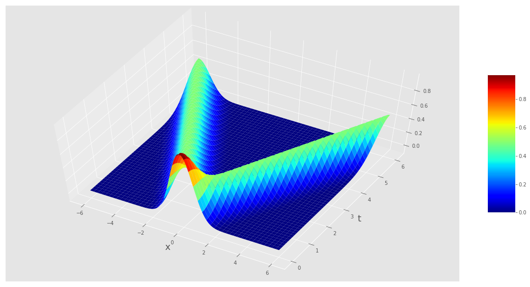
Note the similarities between this plot and the sketches we’ve drawn in lectures when disucssing ideas related to causality.

Gaussian (\(e^{-x^2}\)) initial displacement, sinusoidal initial velocity (\(\frac{1}{10}\sin x\))

Reflection

Suppose we want to solve the wave equation on a semi-infinite string occupying \(x>0\), with initial displacment \(u(x,0)=f(x)=e^{-5(x-2)^2}\) and initial velocity \(u_t(x,0)=g(x)=0\). At the end of the string (\(x=0\)), we fix the displacement to be zero, so \(u(0,t)=0\) for all \(t>0\).

We’ve seen in lectures that the way to tackle this problem is odd reflection, in which we extend the initial conditions by reflecting them in an odd fashion so they’re defined for all \(x\in\mathbb{R}\).

This is shown in the animation below. The first image is a still of the initial condition, so you can see clearly the odd reflection.

Here’s the animation if we let time run:

The solution to the original problem is the restriction of the solution to positive \(x\), i.e. everything to the right of the red line. Everything to the left of the red line is solely a mathematical tool which has allowed us to use d’Alembert’s formula. The odd nature of the reflection ensures that the boundary condition at the string’s endpoint is satisfied.

Click here for an extra example of reflection, with some explanation.